
I found a version of the Mathematica spikey in 3D printable format (STL) at the Shapeways site [1] that was hollow. Here it is when viewed in MeshLab:
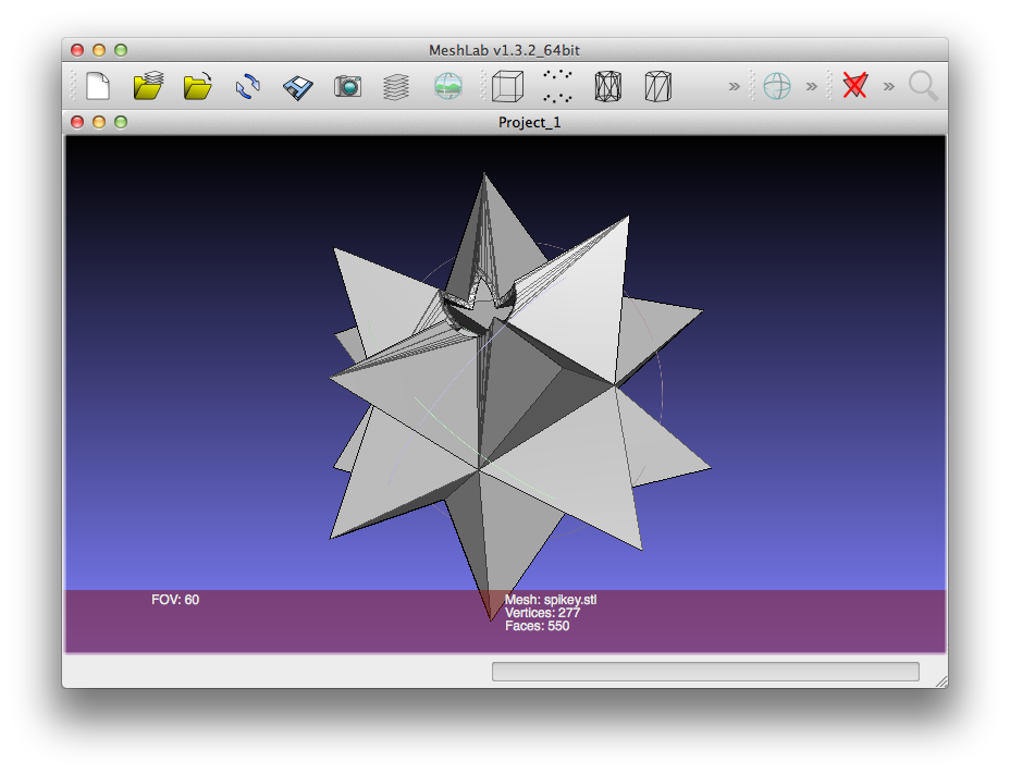
You can see there's a bit cut out of the end, and the whole thing is obviously hollow, with a thick shell.
When I try to make a spikey myself, with code like this:
spikey = PolyhedronData["MathematicaPolyhedron"]
Export["spikey.stl", spikey]
and look at the file in MeshLab, it's solid, but if I look inside, it's obviously just a surface, rather than a thick shell. You can see through to the inside of the opposite faces.
The file with a bite out of it was created by the "Wolfram Team", so I'm pretty sure they used Mathematica. But can this hollowing-out treatment be done using some Mathematica code, or does it require the assembled brain-power of the entire Wolfram organization, or some third-party software, to make polyhedra hollow?
The reason for hollowing out polyhedra is that 3D printers charge per cubic centimeter of material used, so hollow shapes are much cheaper than solid shapes. (This one starts at 45 Euros, so it's quite expensive even when hollow.)
So: How can I hollow out 3D shapes created in Mathematica? Or is it a case of expanding the surfaces to make flat cuboids?
Summary
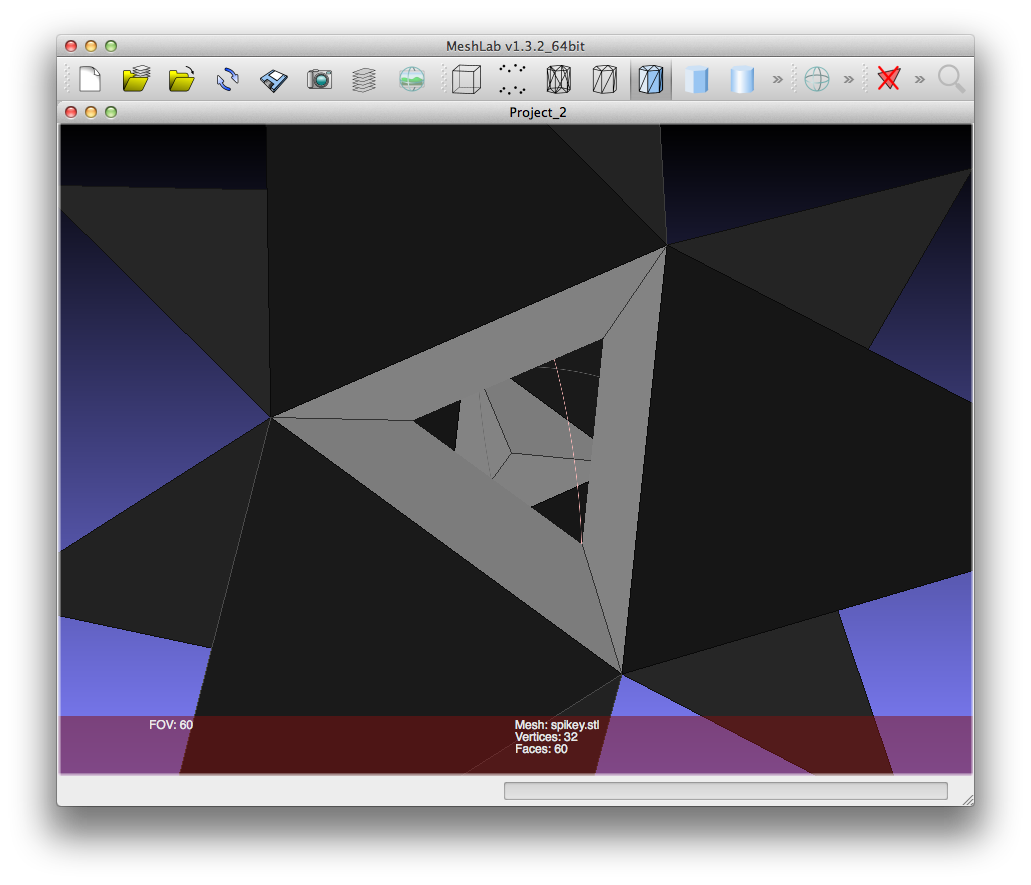
I liked both answers, and in general the solutions work. However, this business of printing 3D polyhedra made in Mathematica proves to be more complicated, and takes me beyond the scope of my innocent initial question. JM.'s excellent thickened polygons look great, but some of the checking programs used by 3D printers consider the adjacent faces to be holes. Here's a picture comparing a cross-section slice of the Wolfram spikey (on the right) with a similar slice through the thickened polygon (on the left):
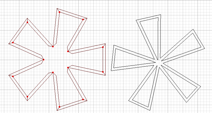
The Wolfram team's version (right) has no internal walls. The adjacent surfaces in the version built by the code on this page (left) are considered to be 'holes' by analysis programs such as NetFabb, even though it makes no visible difference to us. The construction of an interior wall (jVincent's approach) also looks good, and passes some checks (but not others); for printing purposes these shapes should ideally have a hole joining outside and inside surfaces.
I think a future version of Mathematica could benefit from something like Boolean operations for solid shapes, whereby simpler shapes could be merged together to form more complex shapes that are less problematic for subsequent use. Perhaps in version 9.0?! :)
I'm not sure if this will print, but to get a thick wall, you could create a new graphics complex with offset and reversed faces. The surface normal is defined by the traversal direction, so reversing the order flips the normal.
base = Normal[PolyhedronData["MathematicaPolyhedron", "Faces"]];
spikey = Join[base , base /. Polygon[a_List] :> Polygon[Reverse[a] 0.9]];
Export["spikey.stl", Graphics3D[spikey]]
If you need to do some special editing around the base or top, it might be easier to do it manually, but you could also play around with doing it through mathematica prior to exporting it. The method used here (radial expansion) won't work in all cases, but you could properly make a face to wall rule that would work more generally.
 ACCEPTED]
Here's a procedure I use:
(* barycenter of a polygon *)
averagepoints[points_?MatrixQ] :=
        Mean[If[TrueQ[First[points] == Last[points]], Most, Identity][points]]

(* Newell's algorithm for face normals *)
newellNormals[pts_?MatrixQ] := Module[{tp = Transpose[pts]}, Normalize[MapThread[Dot,
              {RotateLeft[ListConvolve[{{-1, 1}}, tp, {-1, -1}]],
               RotateRight[ListConvolve[{{1, 1}}, tp, {-1, -1}]]}]]]

thickenaux[points_, outer_, thick_] := Module[{center = averagepoints[points],
  nrm = newellNormals[points], outerpoints, radialpoints},
  outerpoints = Map[(center - thick nrm + outer (# - center)) &, points];
  radialpoints = MapThread[Join[Reverse[#1], #2] &,
                           Map[Partition[#, 2, 1, 1] &, {points, outerpoints}]];
  Flatten[{Polygon[points], Polygon /@ radialpoints, Polygon[Reverse[outerpoints]]}]]

ThickenPolygons[shape_, outer_: 0.8, thick_: 0.04] :=
 shape /. Polygon[p_?MatrixQ] :> thickenaux[p, outer, thick]
The procedure is more or less a modification of the old (undocumented) package function OutlinePolygons[] in Graphics`Shapes`.
Let's try it out on a simpler case:
Graphics3D[{FaceForm[Cyan, Red], ThickenPolygons[
   Delete[Cases[Normal[PolyhedronData["Tetrahedron"]], _Polygon, Infinity], 3]]},
   Boxed -> False, Lighting -> "Neutral"]

Note that both the interior and exterior are colored with Cyan; this is due to the code ensuring that all the polygons generated are oriented properly.
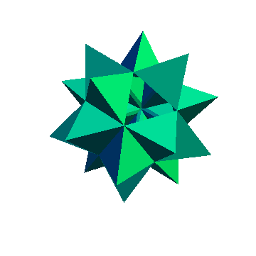
I don't know how to cut a hole in the manner shown in the Shapeways model, so I'll go for a spikey with a simpler cutaway:
Needs["PolyhedronOperations`"];
spikeyCut = Cases[Normal[Stellate[
     MapAt[Delete[#, {1, 4}] &, PolyhedronData["Icosahedron"], {1, 2}],
     1 + 2 Sqrt[7 - 3 Sqrt[5]]]], _Polygon, Infinity];

Graphics3D[{Directive[EdgeForm[], ColorData["Legacy", "SpringGreen"]],
   ThickenPolygons[spikeyCut]}, Boxed -> False]
I set the defaults in ThickenPolygons[] to work for tetrahedra; for other polyhedra or for parametrically-defined surfaces, you might need to play around with the values for the parameters outer and thick.
Here's an alternate version, which might be more suitable for polyhedra than the previous version:
thickenaux[points_, outer_, fac_] :=
 Module[{center = averagepoints[points], nrm = newellNormals[points], n, outerpoints,
         radialpoints, thick},
  n = Length[points] - Boole[TrueQ[First[points] == Last[points]]];
  thick = fac (1 - outer) Mean[Norm[# - center] & /@ points];
  outerpoints = Map[(center - thick nrm + outer (# - center)) &, points];
  radialpoints = MapThread[Join[Reverse[#1], #2] &,
    Map[Partition[#, 2, 1, {1, 1}] &, {points, outerpoints}]];
  Flatten[{Polygon[points], Polygon /@ radialpoints, Polygon[Reverse[outerpoints]]}]]

ThickenPolygons[shape_, outer_: 0.8, fac_: Sqrt[2]/4] :=
 shape /. Polygon[p_?MatrixQ] :> thickenaux[p, outer, fac]
If you run this version of ThickenPolygons[] on spikeyCut and carefully inspect the coordinates, you'll see that the points in the inner walls match up perfectly; there are neither gaps nor unintentional polygon intersections.
The proper value of fac to use will depend on the polyhedron being considered. For the Platonic solids ($\phi$ denotes the golden ratio),
\begin{array}{c|c} \text{polyhedron}&\class{code}{\text{fac}}\\\hline \text{cube}&\frac1{\sqrt 2}\\ \text{dodecahedron}&\frac{1+\phi}{2}\\ \text{icosahedron}&\frac{1+\phi}{2}\\ \text{octahedron}&\frac1{\sqrt 2}\\ \text{tetrahedron}&\frac1{2\sqrt 2} \end{array}
The default value used for fac works for the tetrahedron and the spikey.
In version 11, one has ShellRegion[] that is supposedly useful for 3D printers who want to save on material. Its performance on the spikey leaves something to be desired, tho:
Show[ShellRegion[PolyhedronData["Spikey", "BoundaryMeshRegion"], 1/20],
     BaseStyle -> Opacity[0.5]]

The easiest way I have found to do this is to create the solid model in Mathematica, export it as an STL file, then hollow it out in OpenSCAD. The way you do that is with code like this:
difference() {
  import("spikey.stl");
  scale([.9,.9,.9]) import("spikey.stl");
}
You could then cut a hole in the shell with another difference command.
Import[]the thing in Mathematica:Import["http://www.shapeways.com/model/download/669186", "original-669186_v0.stl"]- J. M.'s missing motivationThickenPolygons[]for your tests? - J. M.'s missing motivation